astropy.table provides functionality for storing and manipulating heterogeneous tables of data in a way that is familiar to numpy users. A few notable capabilities of this package are:
The basic workflow for creating a table, accessing table elements, and modifying the table is shown below. These examples demonstrate a concise case, while the full astropy.table documentation is available from the Using table section.
First create a simple table with columns of data named a , b , c , and d . These columns have integer, float, string, and Quantity values respectively:
>>> from astropy.table import QTable >>> import astropy.units as u >>> import numpy as np >>> a = np.array([1, 4, 5], dtype=np.int32) >>> b = [2.0, 5.0, 8.5] >>> c = ['x', 'y', 'z'] >>> d = [10, 20, 30] * u.m / u.s >>> t = QTable([a, b, c, d], . names=('a', 'b', 'c', 'd'), . meta='name': 'first table'>)
If the table data have no units or you prefer to not use Quantity , then you can use the Table class to create tables. The only difference between QTable and Table is the behavior when adding a column that has units. See Quantity and QTable and Columns with Units for details on the differences and use cases.
There are many other ways of Constructing a Table , including from a list of rows (either tuples or dicts), from a numpy structured or 2D array, by adding columns or rows incrementally, or even from a pandas.DataFrame .
There are a few ways of Accessing a Table . You can get detailed information about the table values and column definitions as follows:
>>> t a b c d m / s int32 float64 str1 float64 ----- ------- ---- ------- 1 2.0 x 10.0 4 5.0 y 20.0 5 8.5 z 30.0
You can get summary information about the table as follows:
>>> t.info name dtype unit class ---- ------- ----- -------- a int32 Column b float64 Column c str1 Column d float64 m / s Quantity
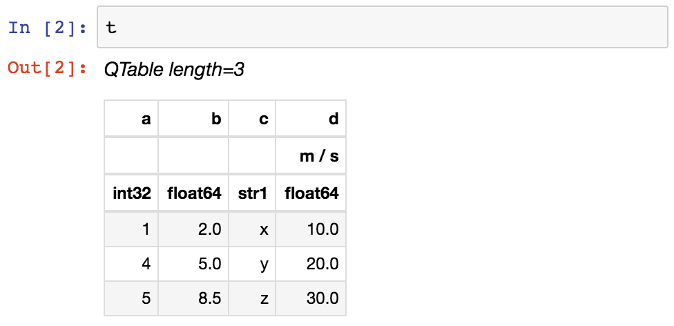
From within a Jupyter notebook, the table is displayed as a formatted HTML table (details of how it appears can be changed by altering the astropy.table.default_notebook_table_class configuration item):
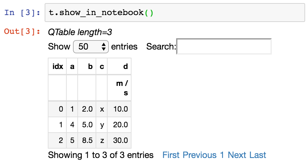
Or you can get a fancier notebook interface with in-browser search, and sort using show_in_notebook :
If you print the table (either from the notebook or in a text console session) then a formatted version appears:
>>> print(t) a b c d m / s --- --- --- ----- 1 2.0 x 10.0 4 5.0 y 20.0 5 8.5 z 30.0
If you do not like the format of a particular column, you can change it:
>>> t['b'].info.format = '7.3f' >>> print(t) a b c d m / s --- ------- --- ----- 1 2.000 x 10.0 4 5.000 y 20.0 5 8.500 z 30.0
For a long table you can scroll up and down through the table one page at time:
>>> t.more()
You can also display it as an HTML-formatted table in the browser:
>>> t.show_in_browser()
Or as an interactive (searchable and sortable) javascript table:
>>> t.show_in_browser(jsviewer=True)
Now examine some high-level information about the table:
>>> t.colnames ['a', 'b', 'c', 'd'] >>> len(t) 3 >>> t.metaAccess the data by column or row using familiar numpy structured array syntax:
>>> t['a'] # Column 'a' 1 4 5 >>> t['a'][1] # Row 1 of column 'a' 4 >>> t[1] # Row object for table row index=1 a b c d m / s int32 float64 str1 float64 ----- ------- ---- ------- 4 5.000 y 20.0 >>> t[1]['a'] # Column 'a' of row 1 4
You can retrieve a subset of a table by rows (using a slice) or by columns (using column names), where the subset is returned as a new table:
>>> print(t[0:2]) # Table object with rows 0 and 1 a b c d m / s --- ------- --- ----- 1 2.000 x 10.0 4 5.000 y 20.0 >>> print(t['a', 'c']) # Table with cols 'a', 'c' a c --- --- 1 x 4 y 5 z
Modifying a Table in place is flexible and works as you would expect:
>>> t['a'][:] = [-1, -2, -3] # Set all column values in place >>> t['a'][2] = 30 # Set row 2 of column 'a' >>> t[1] = (8, 9.0, "W", 4 * u.m / u.s) # Set all row values >>> t[1]['b'] = -9 # Set column 'b' of row 1 >>> t[0:2]['b'] = 100.0 # Set column 'b' of rows 0 and 1 >>> print(t) a b c d m / s --- ------- --- ----- -1 100.000 x 10.0 8 100.000 W 4.0 30 8.500 z 30.0
Replace, add, remove, and rename columns with the following:
>>> t['b'] = ['a', 'new', 'dtype'] # Replace column b (different from in-place) >>> t['e'] = [1, 2, 3] # Add column d >>> del t['c'] # Delete column c >>> t.rename_column('a', 'A') # Rename column a to A >>> t.colnames ['A', 'b', 'd', 'e']
Adding a new row of data to the table is as follows. Note that the unit value is given in cm / s but will be added to the table as 0.1 m / s in accord with the existing unit.
>>> t.add_row([-8, 'string', 10 * u.cm / u.s, 10]) >>> len(t) 4
You can create a table with support for missing values, for example, by setting masked=True :
>>> t = QTable([a, b, c], names=('a', 'b', 'c'), masked=True, dtype=('i4', 'f8', 'U1')) >>> t['a'].mask = [True, True, False] >>> t a b c int32 float64 str1 ----- ------- ---- -- 2.0 x -- 5.0 y 5 8.5 z
In addition to Quantity , you can include certain object types like Time , SkyCoord , and NdarrayMixin in your table. These “mixin” columns behave like a hybrid of a regular Column and the native object type (see Mixin Columns ). For example:
>>> from astropy.time import Time >>> from astropy.coordinates import SkyCoord >>> tm = Time(['2000:002', '2002:345']) >>> sc = SkyCoord([10, 20], [-45, +40], unit='deg') >>> t = QTable([tm, sc], names=['time', 'skycoord']) >>> t time skycoord deg,deg object object --------------------- ---------- 2000:002:00:00:00.000 10.0,-45.0 2002:345:00:00:00.000 20.0,40.0
Now let us compute the interval since the launch of the Chandra X-ray Observatory aboard STS-93 and store this in our table as a Quantity in days:
>>> dt = t['time'] - Time('1999-07-23 04:30:59.984') >>> t['dt_cxo'] = dt.to(u.d) >>> t['dt_cxo'].info.format = '.3f' >>> print(t) time skycoord dt_cxo deg,deg d --------------------- ---------- -------- 2000:002:00:00:00.000 10.0,-45.0 162.812 2002:345:00:00:00.000 20.0,40.0 1236.812
The details of using astropy.table are provided in the following sections:
Constructing Table objects row by row using add_row() can be very slow:
>>> from astropy.table import Table >>> t = Table(names=['a', 'b']) >>> for i in range(100): . t.add_row((1, 2))
If you do need to loop in your code to create the rows, a much faster approach is to construct a list of rows and then create the Table object at the very end:
>>> rows = [] >>> for i in range(100): . rows.append((1, 2)) >>> t = Table(rows=rows, names=['a', 'b'])
Writing a Table with MaskedColumn to .ecsv using write() can be very slow:
>>> from astropy.table import Table >>> import numpy as np >>> x = np.arange(10000, dtype=float) >>> tm = Table([x], masked=True) >>> tm.write('tm.ecsv', overwrite=True)
If you want to write .ecsv using write() , then use serialize_method='data_mask' . This uses the non-masked version of data and it is faster:
>>> tm.write('tm.ecsv', overwrite=True, serialize_method='data_mask')
By default read() will read the whole table into memory, which can take a lot of memory and can take a lot of time, depending on the table size and file format. In some cases, it is possible to only read a subset of the table by choosing the option memmap=True .
For FITS binary tables, the data is stored row by row, and it is possible to read only a subset of rows, but reading a full column loads the whole table data into memory:
>>> import numpy as np >>> from astropy.table import Table >>> tbl = Table('a': np.arange(1e7), . 'b': np.arange(1e7, dtype=float), . 'c': np.arange(1e7, dtype=float)>) >>> tbl.write('test.fits', overwrite=True) >>> table = Table.read('test.fits', memmap=True) # Very fast, doesn't actually load data >>> table2 = tbl[:100] # Fast, will read only first 100 rows >>> print(table2) # Accessing column data triggers the read a b c ---- ---- ---- 0.0 0.0 0.0 1.0 1.0 1.0 2.0 2.0 2.0 . . . 98.0 98.0 98.0 99.0 99.0 99.0 Length = 100 rows >>> col = table['my_column'] # Will load all table into memory
At the moment read() does not support memmap=True for the HDF5 and ASCII file formats.